Using the above technique, a trader can construct the performance distribution based on any performance measure. The trader should choose the performance measure that best reflects his preferences. As an example, consider Rate of Return.

Rate of Return

The most basic performance measure is the Rate of Return. With some types of trading instruments, such as futures, the actual amount of money that must be committed to trading is not clearly fixed. It is therefore convenient to use profit divided by some multiple of maximum drawdown (the largest decline in equity) as a proxy for Rate of Return.

This paper uses profit divided by three times the maximum drawdown. Since maximum drawdown is a measure of risk, this calculation for Rate of Return can also be viewed as risk-adjusted profit. To facilitate comparisons, all figures given in this paper are annualized.

Custom Performance Measures

A trader can combine several existing performance measures into one to better describe his preferences. Here are some measures, in addition to Rate of Return, that traders might want to use:

· Time to recovery. The time from the beginning of a drawdown to the point at which the amount of money in the portfolio is recovered. Can use either the average time to recovery or some other value, such as a high percentile.

· Percent of winning trades. The number of profitable trades divided by the total number of trades (excluding flats).

· Maximum number of consecutive losing trades.

For example, if ROR is Rate of Return and ATR is Average Time to Recovery, performance measure U that best describes a particular trader’s preferences might be:

U=1.0*log ROR-0.5*log ATR (1)

This performance measure basically says that the trader remains indifferent if the Rate of Return increases by 5% while Average Time to Recovery increases by 10%.

If Rate of Return is zero or negative, performance measure U, as written, is meaningless. However, as described in the next section, traders are only interested in a high percentile of the performance distribution, not in the distribution itself. Thus, when Rate of Return is less than some very small positive value (such as 0.01 or 1%), set U to some very negative number (such as -5).

If ROR and ATR change in such a way that performance U remains constant, then the trader is indifferent to this change. At constant U, differentiating equation (1) gives

Since dX/X is approximately the percent change in X, at constant U

This means that the trader remains almost indifferent if Rate of Return increases by some percent while at the same time Average Time to Recovery increases by twice as many percent.

Example: S&P 500 Futures

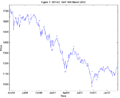
As an example, we do the Random Signals Test for a hypothetical system that trades on S&P 500 March 2002 futures. The data used here is daily closes from 18 March 2000 to 15 March 2002 – 498 trading days in all. Figure 1 shows the price series as well as the signals issued by this hypothetical system.

The hypothetical system produces a profit of 543 points; its maximum drawdown is 126 points. Therefore, its (annualized) Rate of Return is 72%.

The estimated trade characteristics for this system are given in Table 1. The estimation is done by informally combining empirical probabilities with prior beliefs about the system. Transaction cost is roughly based on Wolff’s [2002] slippage estimates. According to Wolff, average slippage in the S&P futures market is between about $140 and $230 per contract round turn. One point in this market is $250.

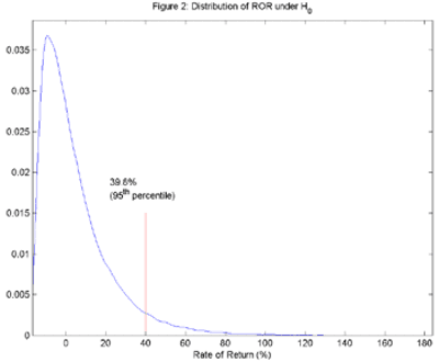
Table 1: Estimated trade characteristics for the hypothetical system whose signals are shown in Figure 1. These parameters are used by the random system to construct the distribution of Rate of Return shown in Figure 2.

We use the estimated trade characteristics from Table 1 to run the random system on the price series. The random system is run 100,000 times. After each run, calculate the Rate of Return. Use these calculations to construct the distribution of Rate of Return under the null hypothesis of random trading. This distribution is shown in Figure 2.

The 95th percentile of this performance distribution is 39.8%. This means that the probability that random trading can achieve a Rate of Return of 39.8% or higher is only 5%. Based on this distribution, the p-value of our hypothetical system is 0.8%(The 95th percentile of profit distribution under the null hypothesis is 433 points. Based on profit, the system’s p-value is 1.9%.).

When only one system is being tested, as is the case here, the p-value is the probability that, given some performance measure, the system is indistinguishable from random trading.

Prof. Alex Strashny

Next: Critical Values

Summary: Index