Let T denote a random lifetime (or time until failure) with distribution function F. On the basis of a sample of n independent replications of T the object of inference are usually

open full size image

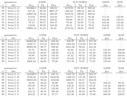
Table 2: Relative efficiency of IFS-based estimator with respect to the empirical distribution function and the kernel density estimator. Small sample sizes.

open full size image

Table 3: Relative efficiency of IFS-based estimator with respect to the empirical distribution function and the kernel density estimator. Moderate sample sizes. quantities derived from the so-called survival function S(t) = 1 − F(t) = P(T > t). If F has a density f then it is possible to define the hazard function

open full size image

and in particular the cumulative hazard function

Usually T is thought to take values in [0,∞), but we can think to consider the estimation conditionally to the last sample failure, say τ and rescale the interval [0,τ] to [0, 1]. So we will assume, from now on, that all the failure times occur in [0,1], being 1 the instant of the last failure when the experiment stops. In this scheme of observation

is a natural estimator of S, with

any estimator of F and, in particular, the IFS estimator. A more realistic situation is when some censoring occurs, in the sense that, as time pass by, some of the initial n observations are removed at random times C not because of failure (or death) but for some other reasons. In this case, a simple distribution function estimator is obviously not good. Let us denote by

the observed instants of failure (or death). A well known estimator of S is the Kaplan-Meyer estimator

where r(t_i) are the subject exposed to risk of death at time t_i and d_i are the dead in the time interval [t_i, t_i+1) (see the original paper of Kaplan and Meyer, 1958, or for a modern account Fleming and Harrington, 1991). In our case d_i is always 1 as t_i are the instants when failures occur. Subjects exposed to risk are those still present in the experiment and not yet dead or censored. This estimator has good properties whenever T and C are independent. Related to the quantities r(t_i) and d_i it is also available the Nelson estimator for the function H

that is defined as

We assume for simplicity that there are no ties, in the sense that in each instant t_i only one failure occurs. The function

is a increasing step-function. Now let

can be thought as an empirical estimates of a distribution function To derive and IFS estimator for the cumulative hazard function H we construct the sample quantiles by simply taking the inverse of

Suppose we want to deal with N +1 quantiles, being

and

One possible definition of the empirical quantile of order k/N is obtained by the formula

(10)

open full size image

for i = 0, 1, ...., d -1 and k = 1, 2,...,N-1 Now set p_i = 1/N, = 1,2,...,N and

as in (10). An IFS estimator of H is

where

is the following IFS:

where

and u is any member of the space of distribution function on [0, 1]. In (10) we have assumed that

is the distribution function of a continuous random variable, with

varying linearly between t_i and t_i+1, but of course any other assumption than linearity can be made as well (for example an exponential behaviour). A Fleming-Harrington (or Altshuler) IFS-estimator of S is then

What is the gain in using our

instead of a standard Altshuler estimator. In principle, it is the same as in distribution function estimation: the Altshuler estimator is a function with jumps and this jumps are smaller with our IFS estimator. But one other important consequence could be the same. Suppose you want to estimate the function h. An estimator is usually given by a discrete density function that gives value d_i/ r(t_i) on t_i and zero elsewhere. The underlying distribution T is a continuous one so we can propose an estimator of its density f by means of the relation h(t) = f(t)/S(t). In fact, let

be the Fourier transform estimator of the density of

Then

is an estimator of h. A density estimator for f is then

or, in alternative, using the Kaplan-Meyer estimator of S

Stefano M. Iacus, Davide La Torre

Next: Final remarks

Summary: Index