Efficiency factors in block designs
As a more complete, if a little pedestrian, example of a function, consider finding the efficiency factors for a block design.
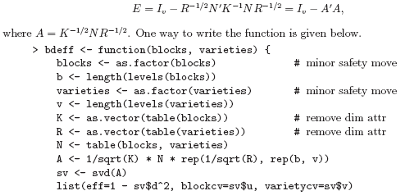
A block design is defined by two factors, say blocks (b levels) and varieties (v levels). If R and K are the v by v and b by b replications and block size matrices, respectively, and N is the b by v incidence matrix, then the efficiency factors are defined as the eigenvalues of the matrix
}
It is numerically slightly better to work with the singular value decomposition on this occasion rather than the eigenvalue routines. The result of the function is a list giving not only the efficiency factors as the first component, but also the block and variety canonical contrasts, since sometimes these give additional useful qualitative information.
Dropping all names in a printed array
For printing purposes with large matrices or arrays, it is often useful to print them in close block form without the array names or numbers. Removing the dimnames attribute will not achieve this effect, but rather the array must be given a dimnames attribute consisting of empty strings. For example to print a matrix, X
> temp <- X
> dimnames(temp) <- list(rep("", nrow(X)), rep("", ncol(X)))
> temp; rm(temp)
This can be much more conveniently done using a function, no.dimnames(), shown below, as a “wrap around” to achieve the same result. It also illustrates how some effective and useful user functions can be quite short.
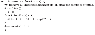
With this function defined, an array may be printed in close format using
> no.dimnames(X)
This is particularly useful for large integer arrays, where patterns are the real interest rather than the values.
Recursive numerical integration
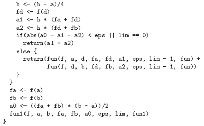
Functions may be recursive, and may themselves define functions within themselves. Note, however, that such functions, or indeed variables, are not inherited by called functions in higher evaluation frames as they would be if they were on the search path. The example below shows a naive way of performing one-dimensional numerical integration. The integrand is evaluated at the end points of the range and in the middle.
If the one-panel trapezium rule answer is close enough to the two panel, then the latter is returned as the value. Otherwise the same process is recursively applied to each panel. The result is an adaptive integration process that concentrates function evaluations in regions where the integrand is farthest from linear. There is, however, a heavy overhead, and the function is only competitive with other algorithms when the integrand is both smooth and very difficult to evaluate. The example is also given partly as a little puzzle in R programming.

Scope
The discussion in this section is somewhat more technical than in other parts of this document. However, it details one of the major differences between S-Plus and R. The symbols which occur in the body of a function can be divided into three classes; formal parameters, local variables and free variables. The formal parameters of a function are those occurring in the argument list of the function. Their values are determined by the process of binding the actual function arguments to the formal parameters.
Local variables are those whose values are determined by the evaluation of expressions in the body of the functions. Variables which are not formal parameters or local variables are called free variables. Free variables become local variables if they are assigned to. Consider the following function definition.

In this function, x is a formal parameter, y is a local variable and z is a free variable. In R the free variable bindings are resolved by first looking in the environment in which the function was created. This is called lexical scope. First we define a function called cube.
cube <- function(n) {
sq <- function() n*n
n*sq()
}
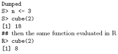
The variable n in the function sq is not an argument to that function. Therefore it is a free variable and the scoping rules must be used to ascertain the value that is to be associated with it. Under static scope (S-Plus) the value is that associated with a global variable named n.
Under lexical scope (R) it is the parameter to the function cube since that is the active binding for the variable n at the time the function sq was defined. The difference between evaluation in R and evaluation in S-Plus is that S-Plus looks for a global variable called n while R first looks for a variable called n in the environment created when cube was invoked.

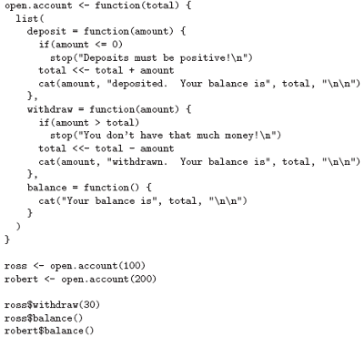
Lexical scope can also be used to give functions mutable state. In the following example we show how R can be used to mimic a bank account. A functioning bank account needs to have a balance or total, a function for making withdrawals, a function for making deposits and a function for stating the current balance. We achieve this by creating the three functions within account and then returning a list containing them.
When account is invoked it takes a numerical argument total and returns a list containing the three functions. Because these functions are defined in an environment which contains total, they will have access to its value. The special assignment operator, <<-, is used to change the value associated with total. This operator looks back in enclosing environments for an environment that contains the symbol total and when it finds such an environment it replaces the value, in that environment, with the value of right hand side.
If the global or top-level environment is reached without finding the symbol total then that variable is created and assigned to there. For most users <<- creates a global variable and assigns the value of the right hand side to it[2]. Only when <<- has been used in a function that was returned as the value of another function will the special behavior described here occur.

Customizing the environment
Users can customize their environment in several different ways. There is a site initialization file and every directory can have its own special initialization file. Finally, the special functions .First and .Last can be used. The location of the site initialization file is taken from the value of the R_PROFILE environment variable. If that variable is unset, the file ‘Rprofile.site’ in the R home subdirectory ‘etc’ is used. This file should contain the commands that you want to execute every time R is started under your system. A second, personal, profile file named ‘.Rprofile’[3] can be placed in any directory.
If R is invoked in that directory then that file will be sourced. This file gives individual users control over their workspace and allows for different startup procedures in different working directories. If no ‘.Rprofile’ file is found in the startup directory, then R looks for a ‘.Rprofile’ file in the user’s home directory and uses that (if it exists). Any function named .First() in either of the two profile files or in the ‘.RData’ image has a special status. It is automatically performed at the beginning of an R session and may be used to initialize the environment.
For example, the definition in the example below alters the prompt to $ and sets up various other useful things that can then be taken for granted in the rest of the session. Thus, the sequence in which files are executed is, ‘Rprofile.site’, ‘.Rprofile’, ‘.RData’ and then .First(). A definition in later files will mask definitions in earlier files.

Similarly a function .Last(), if defined, is (normally) executed at the very end of the session. An example is given below.

Classes, generic functions and object orientation
The class of an object determines how it will be treated by what are known as generic functions. Put the other way round, a generic function performs a task or action on its arguments specific to the class of the argument itself. If the argument lacks any class attribute, or has a class not catered for specifically by the generic function in question, there is always a default action provided. An example makes things clearer.
The class mechanism offers the user the facility of designing and writing generic functions for special purposes. Among the other generic functions are plot() for displaying objects graphically, summary() for summarizing analyses of various types, and anova() for comparing statistical models. The number of generic functions that can treat a class in a specific way can be quite large. For example, the functions that can accommodate in some fashion objects of class "data.frame" include
[ [[<- any as.matrix
[<- mean plot summary
A currently complete list can be got by using the methods() function:
> methods(class="data.frame")
Conversely the number of classes a generic function can handle can also be quite large. For example the plot() function has a default method and variants for objects of classes "data.frame", "density", "factor", and more. A complete list can be got again by using the methods() function:
> methods(plot)
The reader is referred to the official references for a complete discussion of this mechanism.
2 In some sense this mimics the behavior in S-Plus since in S-Plus this operator always creates or assigns to a global variable.
3 So it is hidden under UNIX.
Next: Statistical models in R
Summary: Index