As we have seen informally along the way, the R language allows the user to create objects of mode function. These are true R functions that are stored in a special internal form and may be used in further expressions and so on. In the process, the language gains enormously in power, convenience and elegance, and learning to write useful functions is one of the main ways to make your use of R comfortable and productive.

It should be emphasized that most of the functions supplied as part of the R system, such as mean(), var(), postscript() and so on, are themselves written in R and thus do not differ materially from user written functions. A function is defined by an assignment of the form

> name <- function(arg_1, arg_2, ...) expression

The expression is an R expression, (usually a grouped expression), that uses the arguments, arg i, to calculate a value. The value of the expression is the value returned for the function. A call to the function then usually takes the form name(expr_1, expr_2, ...) and may occur anywhere a function call is legitimate.

Simple examples

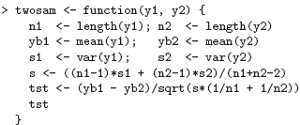
As a first example, consider a function to calculate the two sample t-statistic, showing “all the steps”. This is an artificial example, of course, since there are other, simpler ways of achieving the same end. The function is defined as follows:

With this function defined, you could perform two sample t-tests using a call such as

> tstat <- twosam(data$male, data$female); tstat

As a second example, consider a function to emulate directly the Matlab backslash command, which returns the coefficients of the orthogonal projection of the vector y onto the column space of the matrix, X. (This is ordinarily called the least squares estimate of the regression coefficients.) This would ordinarily be done with the qr() function; however this is sometimes a bit tricky to use directly and it pays to have a simple function such as the following to use it safely. Thus given a n by 1 vector y and an n by p matrix X then X y is defined as (X'X)−X'y, where (X'X)− is a generalized inverse of X'X.

After this object is created it may be used in statements such as

> regcoeff <- bslash(Xmat, yvar)

and so on.

The classical R function lsfit() does this job quite well, and more. It in turn uses the functions qr() and qr.coef() in the slightly counterintuitive way above to do this part of the calculation. Hence there is probably some value in having just this part isolated in a simple to use function if it is going to be in frequent use. If so, we may wish to make it a matrix binary operator for even more convenient use.

Defining new binary operators

Had we given the bslash() function a different name, namely one of the form %anything% it could have been used as a binary operator in expressions rather than in function form. Suppose, for example, we choose ! for the internal character. The function definition would then start as

> "%!%" <- function(X, y) { ... }

(Note the use of quote marks.) The function could then be used as X %!% y. (The backslash symbol itself is not a convenient choice as it presents special problems in this context.) The matrix multiplication operator, %*%, and the outer product matrix operator %o% are other examples of binary operators defined in this way.

Named arguments and defaults

if arguments to called functions are given in the “name=object” form, they may be given in any order. Furthermore the argument sequence may begin in the unnamed, positional form, and specify named arguments after the positional arguments. Thus if there is a function fun1 defined by

> fun1 <- function(data, data.frame, graph, limit) {

[function body omitted]

}

then the function may be invoked in several ways, for example

> ans <- fun1(d, df, TRUE, 20)

> ans <- fun1(d, df, graph=TRUE, limit=20)

> ans <- fun1(data=d, limit=20, graph=TRUE, data.frame=df)

are all equivalent.

In many cases arguments can be given commonly appropriate default values, in which case they may be omitted altogether from the call when the defaults are appropriate. For example, if fun1 were defined as

> fun1 <- function(data, data.frame, graph=TRUE, limit=20) { ... }

it could be called as

> ans <- fun1(d, df)

which is now equivalent to the three cases above, or as

> ans <- fun1(d, df, limit=10)

which changes one of the defaults. It is important to note that defaults may be arbitrary expressions, even involving other arguments to the same function; they are not restricted to be constants as in our simple example here.

The ‘...’ argument

Another frequent requirement is to allow one function to pass on argument settings to another. For example many graphics functions use the function par() and functions like plot() allow the user to pass on graphical parameters to par() to control the graphical output.

This can be done by including an extra argument, literally ‘...’, of the function, which may then be passed on. An outline example is given below.

Assignments within functions

Note that any ordinary assignments done within the function are local and temporary and are lost after exit from the function. Thus the assignment X <- qr(X) does not affect the value of the argument in the calling program. To understand completely the rules governing the scope of R assignments the reader needs to be familiar with the notion of an evaluation frame.

This is a somewhat advanced, though hardly difficult, topic and is not covered further here. If global and permanent assignments are intended within a function, then either the “superassignment” operator, <<- or the function assign() can be used. See the help document for details. S-Plus users should be aware that <<- has different semantics in R.

Next: More advanced examples

Summary: Index