So far we have compared a single sample to a normal distribution. A much more common operation is to compare aspects of two samples. Note that in R, all “classical” tests including the ones used below are in package stats which is normally loaded. Consider the following sets of data on the latent heat of the fusion of ice (cal/gm) from Rice (1995, p.490)
Method A: 79.98 80.04 80.02 80.04 80.03 80.03 80.04 79.97 80.05 80.03 80.02 80.00 80.02
Method B: 80.02 79.94 79.98 79.97 79.97 80.03 79.95 79.97
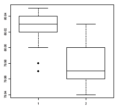
Boxplots provide a simple graphical comparison of the two samples.
A <- scan()
79.98 80.04 80.02 80.04 80.03 80.03 80.04 79.97 80.05 80.03 80.02 80.00 80.02
B <- scan()
80.02 79.94 79.98 79.97 79.97 80.03 79.95 79.97
boxplot(A, B)
which indicates that the first group tends to give higher results than the second.

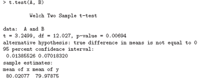
To test for the equality of the means of the two examples, we can use an unpaired t-test by

which does indicate a significant difference, assuming normality. By default the R function does not assume equality of variances in the two samples (in contrast to the similar S-Plus t.test function). We can use the F test to test for equality in the variances, provided that the two samples are from normal populations.
> var.test(A, B)
F test to compare two variances

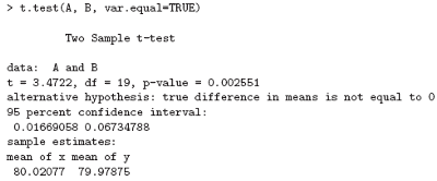
which shows no evidence of a significant difference, and so we can use the classical t-test that assumes equality of the variances.

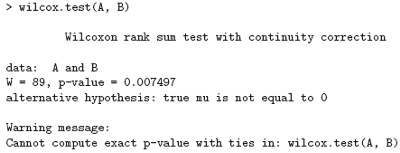
All these tests assume normality of the two samples. The two-sample Wilcoxon (or Mann- Whitney) test only assumes a common continuous distribution under the null hypothesis.

Note the warning: there are several ties in each sample, which suggests strongly that these data are from a discrete distribution (probably due to rounding). There are several ways to compare graphically the two samples. We have already seen a pair of boxplots. The following
> plot(ecdf(A), do.points=FALSE, verticals=TRUE, xlim=range(A, B))
> plot(ecdf(B), do.points=FALSE, verticals=TRUE, add=TRUE)
will show the two empirical CDFs, and qqplot will perform a Q-Q plot of the two samples. The Kolmogorov-Smirnov test is of the maximal vertical distance between the two ecdf’s, assuming a common continuous distribution:


Next: Grouping, loops and conditional execution
Summary: Index