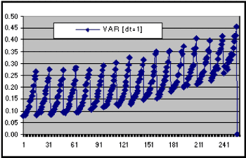
Using the subdivision method from Kloeden described above (page 14) with a big integration step (K = 3000), we can calculate 1, 000, 000 double integrals and separate them into small intervals between the original random numbers Z1 and Z2 (we use them to create our original Wiener process W1 and W2). The purpose is to calculate the mean and the variance of the double integral {24}. And if we plot these results, we find that {24} follows the next variance path:

Figure 2.4.- Real variance path for the double integral {24}.

And if we use:

(39)

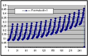
we can see that {39} gives us an exact mirror or representation of the original one:

Figure 2.5.- Mirror of the real variance path for the double integral {24}.

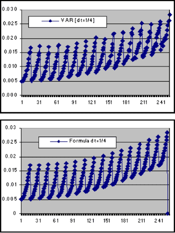
It is the same for dt = 1/4:

Figure 2.6.- Real and Mirror of the variance for the double integral {24}.

Analyzing the numerical results from the simulation (Appendix 2), we can conclude that the double integral {24} has the following mean and variance:

(40)

where:

and, for the Lévy Area, we obtain what we already knew [10]:

On the other hand, if we use the property {27}, we can conclude other properties:

If we assume that the double integrals follow the next SDE:

and using both the properties above and the same criteria of the Fourier formulae (page 16), we define:

(41)

or using the Lévy Area:

(42)

where Z1 and Z2 are the original random numbers of the Wiener process and Z3 is a simple normal distribution random number with mean 0 and variance 1.

We call {41} the Real Variance formulae as it is the best approximation to calculate the right probability of the double integral when compared with all of the methods described above. However, we can not have complete confidence that this is the best method to use because there exists infinite combinations between Z1, Z2, and other independent random numbers that can have the same main properties (future research). For example, we find for dt = 1, which is a special case, the best approximation is:

(43)

and we call this the Fast Variance formulae (dt = 1).

Prof. Klaus Schmitz

Next: Simulation of the Double Integral

Summary: Index