Alphabetical Index of the all other AO Indicators
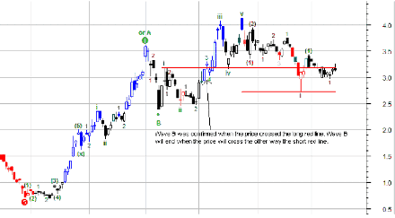
AO (Trig): This indicator is used to show the trigger level of a wave and the required retracement to confirm its end. It has a sensitivity input and is dynamic for the short segment, which is the line that will display at the selected retracement percent applied to the lowest or highest price value since the beginning of that wave. As long as there is no higher or lower value, it will display until the price crosses it giving a confirmation signal; then the short line will be replaced by the long one and a new short will trail the highest or lowest. To know from which value the short segment computes, look at the bar where the short line starts. On bar 1 you will hardly see a dot but as bars go by, the line gets longer.
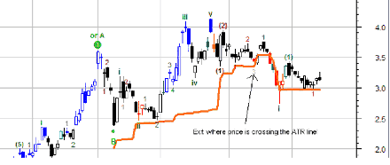
AO ATR Ratchet: This indicator is used to show the stop price level of a transaction initiated at the specified date. It is a self adaptive average that reacts to volatility. The parameters are sensitivity, date, look back periods and acceleration factor. Shown below is the ratchet at 34%, note it does not disappear after a violation so it must be removed when no longer needed.
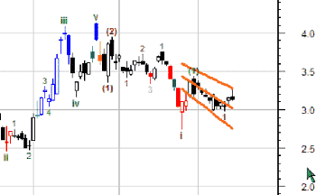
AO Auto Fib Fan: This indicator will plot the Fibonacci fan price levels for the previous peak or trough of specified sensitivity. It is automatic so when the wave of the selected sensitivity is over and confirmed, it will switch direction, thus always providing a Fibonacci fan at 38.2%, 50% and 61.8% of the slope.
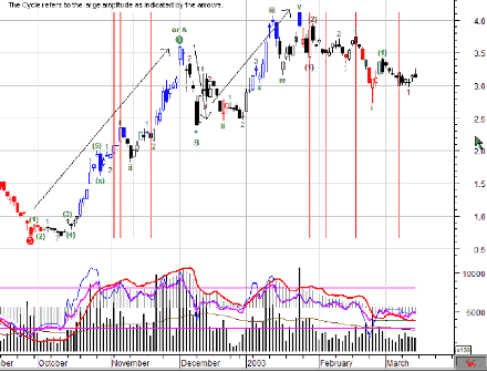
AO Auto Fib Time (P): This indicator will plot the Fibonacci Cycles based on the previous peak or trough (specified sensitivity) on the price window. Again the 38.2%, 50%, 61.8% and 100% ratios are used. This indicator is intended for the price pane and should be displayed as a histogram using no scale so it floats freely.
AO Auto Gann Angles: This indicator plots automatically the Gann angles for the specified sensitivity. Here we selected the 34% sensitivity and where the lines reach zero, they become flat to avoid displaying negative values that would compress the rest of the chart.
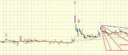
To visualize the starting point and the accuracy, you can superpose Gann Angles from Equis over AlphOmega. Here is an example…
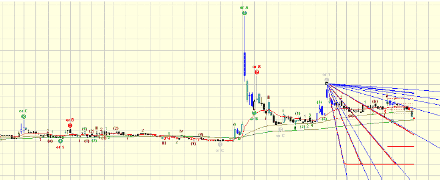
Note that the useless information is automatically discarded, that is only the angles containing the pattern are displayed. Once the pattern moves out of the Equis middle projection, it becomes another pattern.
Next: Appendix 5
Summary: Index